Filtering Algorithms (UKF)

In the first quarter of my graduate program, I took a course on machine learning and artificial intelligence for robotics. All major coding assignments were programmed in Python. This page highlights one project completed throughout the course.

Project 1: Filtering Algorithms

For this project, we provided datasets from a robot platform performing mobile navigation while visually observing landmarks. The ground truth positions for the landmarks were known and were provided for consideration during the measurement update. The robot was freely roaming throughout the environment without any occlusions.

Tasks

The first part of this project focused on generating a motion model. The second part of this project generated a measurement model. Finally, these two were combined with a filtering algorithm. I implemented a Unscented Kalman Filter.

Motion model dead-reckoning

The motion model tested using the commands from Odometry.dat. The results of the entire simulated dataset compared to the groundtruth data is shown in Figure 2. Figure 3 shows the first 10,000 control commands to declutter the scene. Although in Figure 2 it is difficult to tell if the robot is following the correct trajectory, the trajectory in Figure 3 shows that initially the robot is following the same path as the groundtruth data, but without any corrections, the robot veers off course.

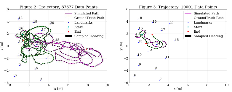
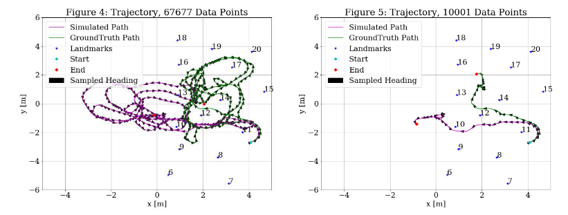
Figure 4 starts from a different groundtruth location. This time, from the 20,000th time step in the groundtruth data. Figure 5 shows the first 10,000 control commands to de-clutter the scene. Again, the Figure 5 shows that initially the robot is following the same path as the groundtruth data, but without any corrections, the robot veers off course.

Unscented Kalman Filter (UKF)

The Unscented Kalman Filter uses sigma points to methodically sample and filter nonlinear systems. At a high level, the UKF takes a position represented by a mean vector and covariance matrix. It then selects a fixed number of samples (2n+1) to represent the possible positions of the object. Weights are assigned to these samples corresponding to how likely they are to be the “true” position. The object is passed through the motion model, then the likely position and covariance are “updated” using these weights. This is the new posterior unless measurement data is available. If there is measurement data, a new selection of (2n+1) samples are then selected from that “updated” belief. Those samples are then passed through the sensor model. A new belief is then calculated using the predicted sensor data, the true sensor data, the prior belief, the samples, the weights, and noise. The algorithm then returns the new belief (mean vector and covariance matrix), which can be passed through the algorithm again if more control and/or sensor data is available.

My interpretation of the algorithm is shown in the flow chart below. After the flow chart, the inputs, outputs and parameters for the overall UKF as well as the sub-modules are listed.

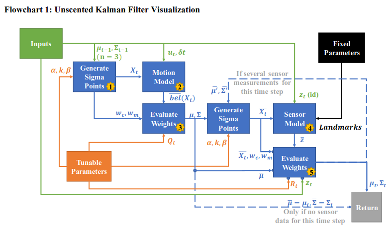
This Unscented Kalman Filter Algorithm is based on the algorithm presented in Table 3.4, pg 70 of Probabilistic Robotics [2]. Wan’s paper on the Unscented Kalman Filter was also referenced to better understand the UKF [3]

Filter implementation

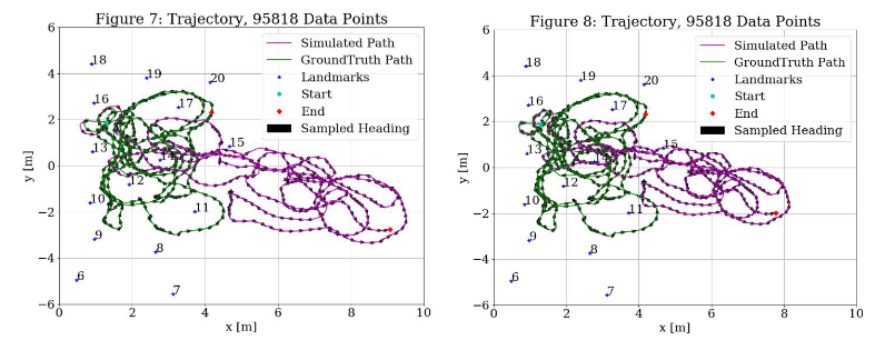
I phased the implementation of the UKF to ensure I understood what was being controlled by each step. First, I ran the UKF through module 3 with 𝑄𝑡 =diag(0,0,0) (i.e. no noise) to compare the result to the plots from section A.3. Due to the lack of noise, the matrix square root had to be computed with the slower, sqrtm function. By inspection, Figure 7 is the same as Figure 3. Then, I added white noise to the filter with 𝑄𝑡 =diag(1,1,1), which slightly changed the shape of the trajectory as is shown in Figure 8

Then, I added in the measurement model with 𝑅𝑡 = diag(1,1). By inspection of Figure 9, the addition of the sensor model clearly improved the trajectory, as the simulated path now stays within the range of the landmarks. The scene is so crowded that it is difficult to see what is happening, so Figure 10 plots the same parameters as Figure 9, but only displays the first 30,000 samples. Figure 10 shows 3X the number of samples as Figure 3. Although the trajectory might not totally match up, the end point is consistent.

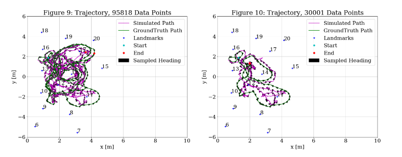
Then, I probed other starting points. Figures 11 and 12 repeat the variables from Figure 10 with starting points 20,000 and 60,000 respectively. These look even better fit than Figure 10.

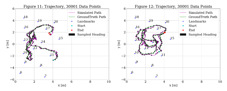
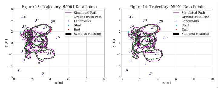
Since Figures 11 and 12 looked better than Figure 10, I then shifted around the start point to see if there were errors coupled to where the data was starting. Figure 13 shows the trajectory starting at 300 instead of 0. This trajectory looks much better than starting as 0, so it will be accepted as the new baseline for tweaking parameters.

Using the lessons learned from the measurement model testing, I decided to screen measurements. I ignored the following: all measurements from 8 and 19, measurements with range >3 for 6-9, and measurements >6 for the rest. As shown in Figure 14, this smoothed the trajectory.

References

1. S. Russell and P. Norvig, Artificial Intelligence: A Modern Approach, 3 ed., Prentice Hall/Pearson Education, 2009, p. 616.
2. S. Thrun, W. Burgard and D. Fox, Probabilistic Robotics, MIT Press Books, 2005.
3. E. A. Wan and R. v. d. Merwe, “The unscented Kalman filter for nonlinear estimation,” , 2000. [Online]. Available: https://seas.harvard.edu/courses/cs281/papers/unscented.pdf. [Accessed 14 10 2019].