Machine Learning (GMM-GMR)

In the first quarter of my graduate program, I took a course on machine learning and artificial intelligence for robotics. All major coding assignments were programmed in Python. This page highlights one project completed throughout the course.

Project 3: Machine Learning

The learning aim of this assignment is learning the measurement model from the filtering project link. The dataset contains the robot location (heading/x/y), the landmark location (x/y), and the measurement between the two (range/bearing). The measurement between the two for the training data was calculated based on the sensor model presented in Chapter 25 pg 980 of Artificial Intelligence [1]. Each row in the learning dataset corresponds to a timestep with measurement data provided with ds0, so the measurements can be used for comparison.

The learning dataset is comprised of 80% of the datapoints in the entire dataset. 20% of the datapoints were reserved for testing. Points were randomly assigned to either the learning dataset or the testing dataset. At the same time, the measurement data was split up between learning and test datasets to facilitate algorithm evaluation. The testing dataset was then split into inputs and outputs. The training input dataset contains the robot location and landmark location. The training output dataset contains the measurement data.

For this project, I decided to learn the measruement model with Gaussian Mixture Model and Gaussian Mixture Regression (GMM-GMR). Each output is the result of an operation on a subset of the inputs. There is clearly a correlation between the inputs and the outputs, so I thought a GMM should be able to reveal that relationship. One concern is the mixture of angles and distances in the formulation, but I address the workaround I used in the next section.

Learning Algorithm

Gaussian mixture models are often used in pattern recognition and machine learning [2]. For this assignment, the GMM was implemented using the expectation maximization (EM) algorithm.
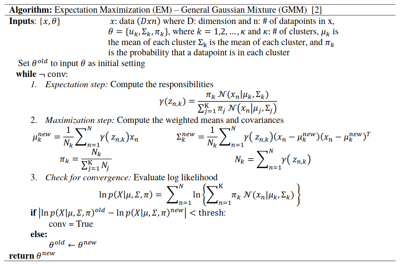
The EM algorithm listed below is specific to Gaussian Mixtures and is based on the algorithm presented in Chapter 8.5 of ESL [2] . The EM algorithm takes the initial “guesses” for the mixing coefficient and distribution for each Gaussian (𝑘). The first step (aka the expectation step, the E in EM) computes the responsibilities/conditional probabilities of 𝑧𝑘 given x. The second step (aka the maximization step, the M in EM) computes the weighted means and covariances given that responsibility and the data. In the EM algorithm, the mixing coefficient 𝜋𝑘 serves the role of the prior probability of 𝑧𝑘 = 1.

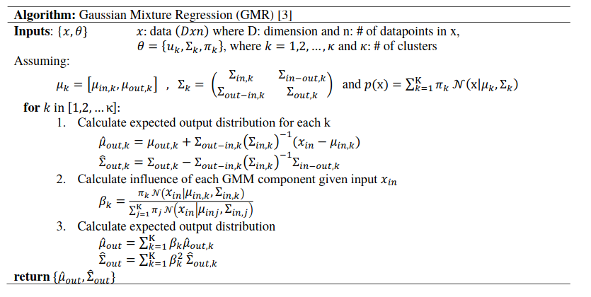
The second part of GMM-GMR is Gaussian mixture regression. Once a model is found, it can be evaluated with GMR. GMR assumes the data is organized such that 𝑥 = [𝑥𝑖𝑛, 𝑥𝑜𝑢𝑡], so means and covariances are separable as shown in the algorithm. The algorithm below is based on Table 59.2 in Robot Programming by Demonstration [3].

Testing

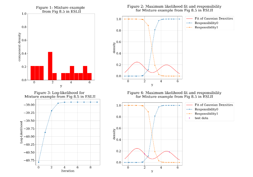
To make sure the algorithm was working properly, I started out by testing the 1D mixture example from Chapter 8.5 of ESL [2]. Figures 1-4 below show the results. Figure 1 shows a histogram of the dummy data. Figure 2 shows the maximum likelihood fit of the Gaussian densities (shown in red) overlaid with the responsibilities of each component density for observation y as a function of y. Figure 3 shows the value of the log-likelihood of the model after each iteration and ultimately shows convergence. Figure 4 shows the results of using GMR to evaluate two new data points. I arbitrarily chose the starting points for this example.

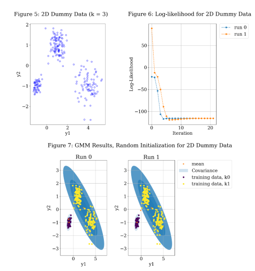
Next, I tested a 2D mixture example generated from sampling three Gaussian distributions. Figures 5-7 shows the results of this testing. Figure 5 shows the input data. Now that the data is 2D, the actual data is plotted on the x and y axes instead of requiring a histogram. Figure 6 shows the value of the log-likelihood of the model after each iteration and ultimately shows convergence. Figure 7 shows the 2D GMM results, where the orange stars are the mean of each component and the blue shaded circles show the covariance (successive circles show several deviations away from the mean). The coloring of the datapoints indicates which Gaussian they are associated with. This was accomplished by using classification instead of regression. The figure shows the result of two different runs, with the seeds of each Gaussian initialized by random selections from the dataset. Even though k = 3, one of the components ends up being so significant that it does not show up in the results. This demonstrates that the GMM is highly dependent on the starting parameters and only guarantees convergence to a local maximum.

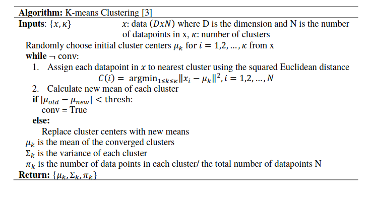
To choose the starting seeds more cleverly, I then implemented the k-means algorithm to initialize the algorithm. The k-means algorithm is seeded with random means for each Gaussian chosen from the data set. Then, each data point in the set is assigned to the nearest mean according to the Euclidean distance from each mean. Once each datapoint is assigned, to a cluster, the mean of each cluster is calculated. This process is repeated until the means converge. The algorithm below is base on the k-means clustering algorithm presented in Chapter 9.1 of Pattern Recognition and Machine Learning [3].

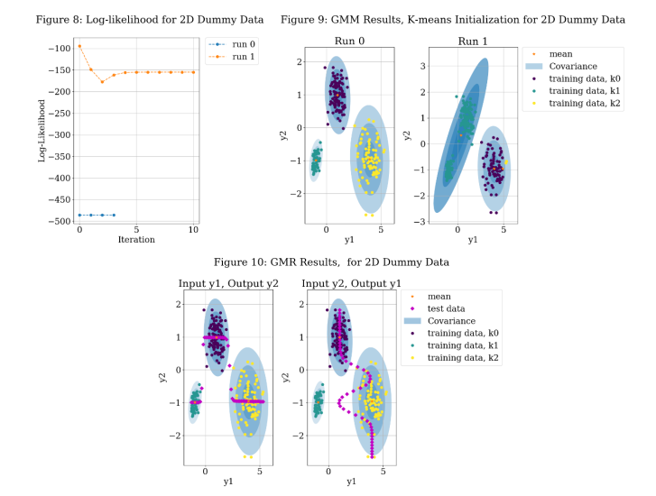
Figures 8-10 use the dataset shown in Figure 5, but the algorithm uses k-means for initialization. Figure 8 shows the value of the log-likelihood of the model after each iteration and ultimately shows convergence. By comparing the result to Figure 6, the algorithm converges more quickly. Visually, you can also see that the two runs converge to different values. Figure 9 shows the 2D GMM result. Run 1 shows only two components, but Run 0 captures all 3. Due to the dependence on the initialization points even with k-means initialization, several run will be completed with different starting point. The one with the lowest least squared error will be selected to plot the GMR results. Figure 10 shows the GMR results for randomly generated test points with each component serving as the input. Visually, it appears that the output is well fit to the data.

I also tested the algorithm on 2D data that needed to be normalized to check the GMR implementation. Those results were plotted on Figures 11-14, but the figures are excluded from this report for brevity. The code still plots these figures, and they are saved in the code submission, so there is a gap in numbers here.

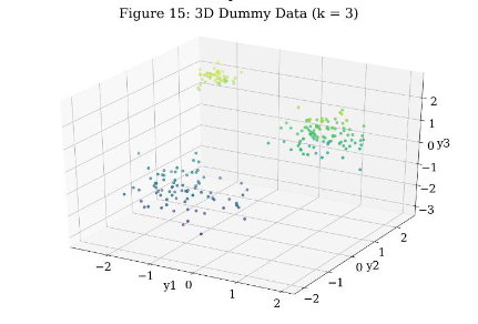
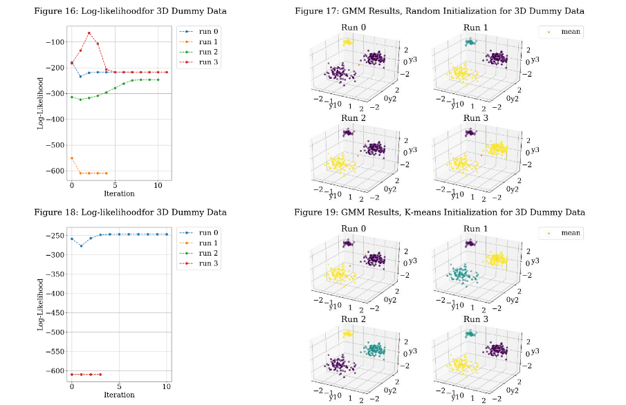
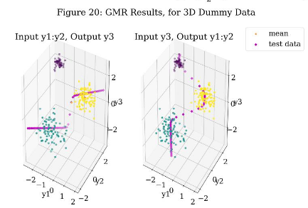
Next, I tested a 3D mixture example generated from sampling three Gaussian distributions. The results are shown in Figures 15-20. Figure 15 shows the dataset in 3D. The coloration is meant to help interpret depth. Figure 16 shows the value of the log-likelihood of the model after each iteration and ultimately shows convergence for random initialization. Figure 17 shows that only Run 1 of the random initialization runs converge to the three Gaussians. Again, classification was used to group the data into Gaussians of color purple, blue, and yellow. The covariance was not plotted for 3D, as it made it difficult to interpret the results. Figure 18 shows the value of the log-likelihood of the model after each iteration and ultimately shows convergence for k-means initialization. Figure 19 shows that all but Run 0 of the k-means initialization runs converge to the three Gaussians. Figure 20 shows GMR for a k- means initialized model. Visually, it appears that the output is well fit to the data

Algorithm Application to Learning Aim (Learning the Measurement Model)

My learning aim is 7D with 5D input and 2D output. Much time was spent on 1D, 2D, and 3D examples up until this point because they are possible to visualize. This is not true for the 7D data. Instead, we will rely on the log- likelihood and mean-squared error for indication of model convergence. This also means that the k-clusters will have to be determined by trying many different values, since we cannot gain insight into the clustering by visualizing the data.

The dataset includes two angles. There are variants of the GMM that account for wrapping called the Wrapped Gaussian Mixture Model (GMM) or the simplified Semi-Wrapped Gaussian Mixture Model (SWGMM) [3]. Rather than implement one of these variants, I decided to linearize the angles by replacing each 𝜃 column with sin(𝜃) and cos (𝜃) columns. This has the disadvantage of adding 2 more dimensions (9D with 6D input and 3D output), but I decided this was preferable to increasing the complexity of the GMM. During GMR, the sin(𝜃) and cos (𝜃) columns in the output are converted back to angles.

Figures 21-30 show the training results for the log-likelihood and mean-squared error for 𝑘 = [1, 2, 3, 6, 10]. The minima mean-squared error results are also summarized in Table 1. Each range and bearing was compared against two values: 1) the geometry-derived result, which was used for training and 2) the measurement data provided with the datasets.

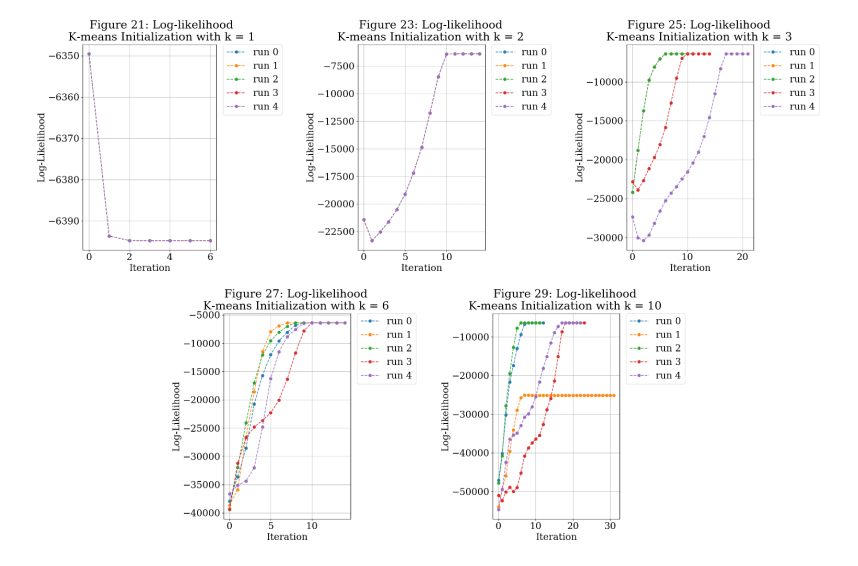
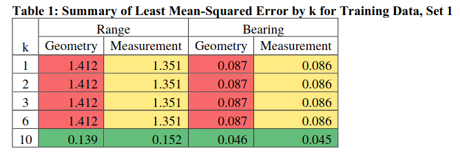
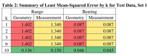
For both the geometry and the measurement, it is clear that k = 10 has a result that outperforms the other models on the training data. Typically, you would just take the “best” result after training the model and use it for the test data. I ran each model on the test data to see if any of the models were over-fit to the training data and would fail with the test data, particularly for Run 1 for k = 10. By inspection, the results of running the test data are closely aligned to the training data. The results are also summarized in Table 2.

References

1. S. Russell and P. Norvig, Artificial Intelligence: Prentice Hall, 2009, p. 616.
2. T. Hastie, R. Tibshirani and J. Friedman, The Elements of Statistical Learning, 2 ed., Springer, 2009.
3. A. . Roy, S. K. Parui and U. . Roy, “SWGMM: a semi-wrapped Gaussian mixture model for clustering of circular—linear data,” Pattern Analysis and Applications, vol. 19, no. 3, pp. 631-645, 2016.
4. R. Misra, “Towards Data Science,” Medium, 11 February 2019. [Online]. Available: https://towardsdatascience.com/inference-using-em-algorithm-d71cccb647bc. [Accessed 8 November 2019].
5. A. Billard, S. Calinon, R. Dillmann, S. Schaal, B. Siciliano and O. Khatib, “Robot Programming by Demonstration,” in Springer Handbook of Robotics, Berlin, Heidelberg, Springer Berlin Heidelberg, 2008, pp. 1371-1394.
6. C. Bishop, Pattern Recognition and Machine Learning, New York: Springer-Verlag, 2006.