Search and Navigation (A*)

In the first quarter of my graduate program, I took a course on machine learning and artificial intelligence for robotics. All major coding assignments were programmed in Python. This page highlights one project completed throughout the course.

Project 2: Search and Navigation

The focus of this project was on the implementation of an A* variant, able to generate 2­D paths that navigate between start and goal locations while avoiding obstacles, and a simple controller that enables a wheeled mobile robot to drive the generated paths.

Environment

• Obstacles: The landmarks (same as project 1).
• Partial observability: The robot is only able to observe obstacles located within its 8 neighbor cells.
• Connectivity: The 8 cells surrounding a given cell are its neighbors. (And theses are the only allowable cell transitions.)
• True cost: +1 to move into a neighbor cell that is unoccupied, +1000 to move into a neighbor cell that is occupied.

A* Algorithm Implementation

A* is an informed search algorithm that applies a best-first search strategy. The algorithm implemented in this homework is based on Section 3.5.2 of Artificial Intelligence [1]. The algorithm is initialized with a starting location, a goal, a map of obstacles, an open set, and a closed set. The open set contains every node that was evaluated minus the nodes that were visited. Each row in the open set contains a node, its cost, and its originating node/prior. The closed set contains all nodes that were visited. Each row in the closed set contains a node and its prior. Allowed actions are +/- one cell in any direction – including diagonally.

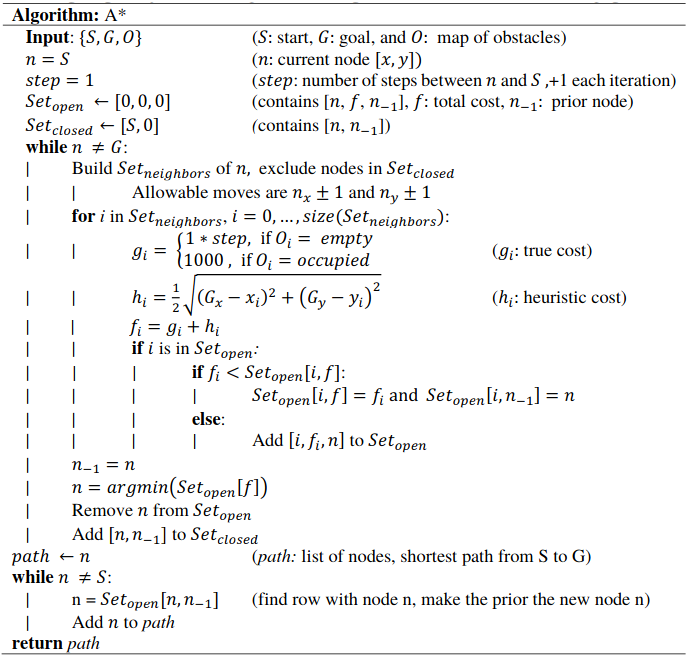
From an initial state, the algorithm selects neighboring nodes using the allowed actions, but skipping any nodes that are already in the closed set. It then assigns a cost to each neighbor. The cost is the sum of the true cost and the heuristic cost. The true cost is the number of steps the neighbor node is away from the starting node. Initially, the heuristic cost was set to be the straight-line distance from the neighbor node to the goal, but this may not be admissible since diagonal moves are allowed. For example, the straight-line path from start to goal for Path C in Although the heuristic may not be admissible, it is complete and optimal for A* offline.

According to Chapter 3 of Artificial Intelligence, we really want our heuristic to be consistent since we are implementing graph-search rather than tree-search [1]. The distinction between tree-search and graph-search is that is that tree-search considers all possible paths to the solution, while graph-search does not consider redundant paths. As is discussed in the next paragraph, we ensure the optimal path to the successor node is found by maintaining a list all nodes evaluated. That being said, to force the heuristic to be admissible for A* offline, the heuristic was updated to be half the straight-line distance from start to goal.

Then, each neighbor is compared to the open set. If the neighbor is listed, the new cost is compared to the old cost. If the new cost is lower, then the cost and prior are updated in the open set. If the neighbor is not listed, then it is added. Then, the node on the open set with the lowest cost is selected to be new starting node. It is removed from the open set and added to the closed set. This process of expanding the sets is repeated recursively until the starting node is the goal. At the end, the closed list is used to trace the shortest path back from the goal to the start.

A* Online Algorithm Implementation

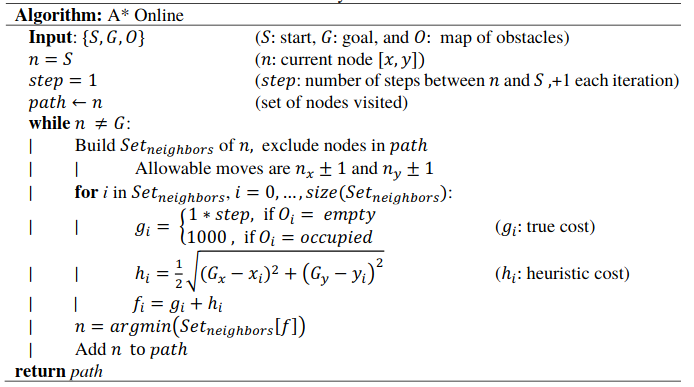
The algorithm was modified to run “online”. Now that the robot cannot observe the obstacle until it encounters it, there is no benefit to planning beyond the next node. Additionally, the robot can only move one cell at a time, so the open set only needs to contain the neighbor nodes. The closed set is now equivalent to the path, so nodes are added directly to the path rather than to an intermediate closed set.

An advantage of running A* online is that the algorithm runs much faster because it no longer needs to maintain a running list of open nodes. This is less noticeable in the Coarse Grid, but I tried running the offline A* algorithm on the Fine Grid that is introduced in A.6, and the it took ~50x longer to find the path than with the A* online. This demonstrates the tradeoff between optimality (offline) and speed (online).

A* Testing

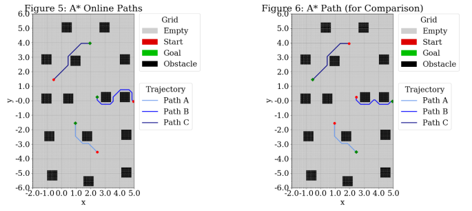
Figure 5 (below) shows the A* designated path from start to goal. For paths A and C, the robot appears to take the optimal path even though it is running A* online and it encounters an obstacle. Path B does not take the optimal path. If A* was running offline, the robot would go “down” around the obstacles. The robot does not have enough information to do this when running A* online because it cannot observe obstacles until it encounters them. I ran the simulation for A* offline to confirm the optimal path matches this description. The result is shown in Figure 6.

Inverse Kinematics Controller

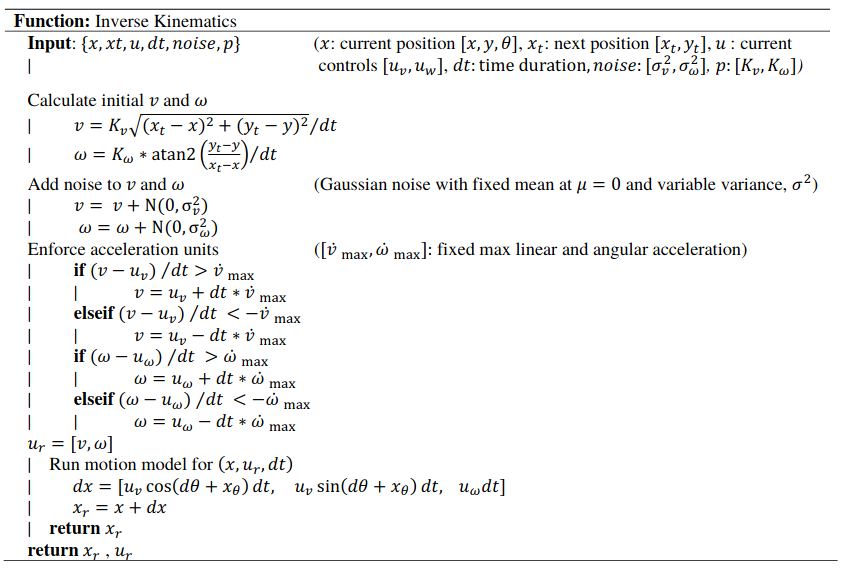
Next, an inverse kinematics controller was implemented for a more realistic comparison of traidtional (offline) A* to A* online. The algorithm is listed below.

Inverse Kinematics Controller Testing

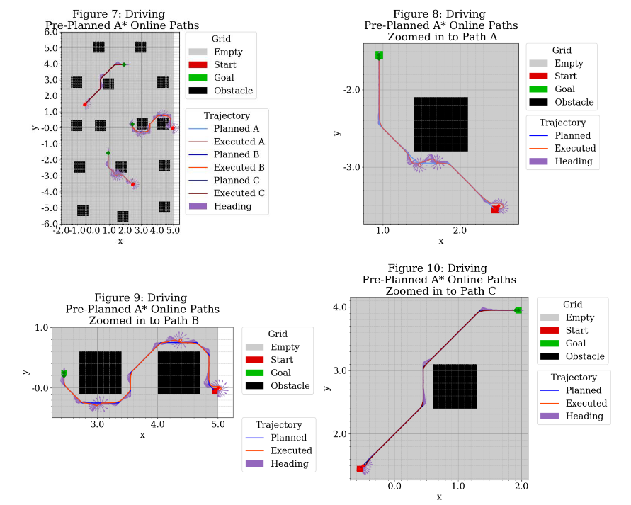
This controller was used to drive “pre-planned” paths specified by A* .To execute the pre-planned path, the inverse kinematics were run recursively for each node until a threshold was reached. Once the threshold was reached, the next node was set as the new goal. I tried tweaking the threshold and found that the larger the threshold, the smoother the trajectory with the caveat that if the threshold was larger than the cell size, then the robot never actually made it to the goal. By smoother, I mean that the robot “cut corners” on the A* path. One consequence of this was that the robot sometimes cut into the obstacles as well. I ended up choosing a threshold of 0.05 to ensure the robot made it into the goal cell.

Below, Figure 7 shows the trajectories. Figures 8, 9, and 10 provide a zoomed-in look at the trajectories. Blue lines indicate planned trajectories, red/orange line specify executed trajectories, and purple arrows indicate heading. Path B had the most difficulty maintaining the desired trajectory. Initially, I thought this was just due to noise, but it remained persistent across many runs. The kinematic model seems to have a hard time traversing the horizontal distances between the start and goal. My best bet is that the p controller tuning I ended up with was optimized for the vertical stretches over the horizontal stretches.

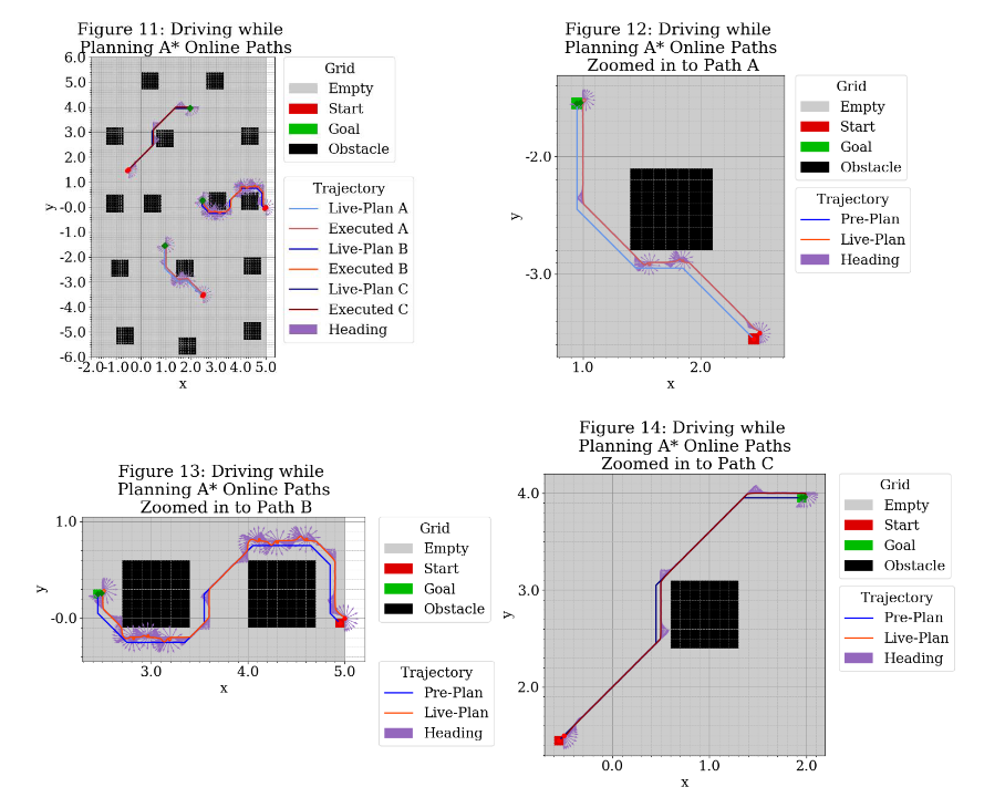
Finally, I used A* Online to “plan while driving” with the inverse kinematic controller. Below, Figure 11 shows the trajectories. Figures 12, 13, and 14 provide a zoomed-in look at the trajectories. Blue lines indicate planned trajectories, red/orange line specify executed trajectories, and purple arrows indicate heading. I noticed that the robot sometimes collided with the obstacles. This collision was typically 1 cell deep, so I increased the buffer around the obstacles by 0.1 to prevent robot from colliding with or riding along the edge of the obstacles. (I only added nodes to the “flat sides”, essentially turning the obstacles into circles.)

Real-world considerations

With the kinematic controller, an additional buffer was added to the obstacles to ensure the robot didn’t hit the obstacle when looping back/reacting to noise. In a real robot, you would want a better understanding of the noise sources in your robot to determine what buffer is really required and what noise thresholds are actually realistic. Having a better understanding of the noise would also help tune the p-controller in a manner that was more informed. Depending on the behavior, it also might be worth implementing a more complicated controller.

Another concern with the kinematic controller could be turning. Although in this simulated setup it wasn’t a concern, it might be an issue for a real robot. It could be advantageous to take a longer path that requires fewer turns, which is essentially what a coarser grid would do. The fine grid (show here) gets as close to the obstacles as possible (as is required with the constraints provided and A* online), so it must make many more turns to navigate around the obstacles. This assignment placed no requirement on total time, but in reality, you might care about how fast the robot gets to a destination more than what the total path was. Additional turns could cause the robot to take longer to reach the goal.

A blended approach which uses coarse and fine grids in difference scenarios would probably be the ideal approach. For this assignment, we said the robot could only see obstacles 1 cell away. In reality, the distance within which the robot could see obstacles would be tied to the sensors that are used. If the sensor is able to see further than 1 cell away, the robot should consider that information. That could help the robot choose which direction to go around an obstacle and give more warning when an obstacle is coming to re-plan.

References

1. S. Russell and P. Norvig, Artificial Intelligence: A Modern Approach, 3 ed., Prentice Hall/Pearson Education, 2009, p. 616.